Dynamic Merkle-Trees


Author: Herman Schoenfeld
Version: 1.1
Date: 2020-01-01 - 2020-10-23
Copyright: (c) Sphere 10 Software Pty Ltd. All Rights Reserved.

Dynamic-Merkle-Trees.pdf

Original e-print
Abstract

This paper presents a formal construction of dynamic merkle-trees and a deep-dive into their mathematical structure. In doing so, new and interesting artefacts are presented as well as novel security proof constructions that enable proofs for a full range of tree transformations including append, update and deletion of leaf nodes (without requiring knowledge of those nodes). Novel concepts are explored including "perfect trees", "sub-trees", "sub-roots" and "flat coordinates" through various lemmas, theorems and algorithms. In particular, a "flat-tree" implementation of merkle-trees is presented suitable for storing trees as a contiguous block of memory that can grow and shrink from the right-side. Of note, a "long-tree" implementation is presented which permits arbitrarily large tree construction in $ O(\frac{1}{2} \log_2N) $ space and time complexity using a novel algorithm. Finally, a reference implementation accompanies this paper which contains a fully implemented and thoroughly tested implementation of dynamic merkle-trees.

1. Introduction

Merkle-trees are a cryptographic construction that enable a collection of objects to be hashed together in a way that preserves information about their individual membership within the collection. Merkle-trees permit statements about the collection, and their objects, to be verified without knowledge of the entire set of objects but only of the objects in question. This is achieved through formally constructed security proofs. The ability to verify statements about the tree without needing to store (or have knowledge) of the tree is the primary innovation and essential purpose of merkle-trees. For example, proving that a leaf-node exists within a merkle-tree requires knowing only the root, the leaf and the path from that leaf to the root. The path here comprises an "existence-proof" of the leaf in the tree. The verifier can cryptographically prove the existence of the leaf in the tree by evaluating the hash-path and comparing the end result with the known root. If it matches, the object is a leaf of the tree.

This initial idea was originally proposed [1] by Ralph Merkle for the specific purposes of overcoming the limitations of "one-time keys" in the Lamport/Winternitz digital signature schemes. He found he was able to transform a "one-time" scheme into a "many-time" scheme by encoding multiple one-time keys as leaves in a merkle-tree. The root of the tree served as the many-time key which represented a cryptographic commitment to all the one-time keys (the leaf nodes). Each signature chose a one-time key and provided an existence-proof of that key along with the digital signature signed by that key. By choosing different one-time keys for each signature, the one-time signature scheme thus transformed into an equivalent many-time scheme.

Since that time, merkle-trees have found a wide domain of applicability. Whilst primarily used in cryptography, many areas of computer science utilize merkle-trees including database management systems, certificate management, peer-to-peer file streaming, blockchains, distributed ledger technology many other established and emerging fields.

This paper extends the primary utility of merkle-trees not just with new proofs for membership and consistency but with general purpose leaf-set transformations including update, delete, append, insert, to name a few. These proofs are sufficient to compose all general leaf-set transformations. Also, a "flat coordinate scheme" for merkle-trees is provided that allows addressing of nodes in a 1-dimensional contiguous block of memory suitable for unbounded trees. Of particular achievement is a tree implementation with $ O(\frac{1}{2} \log_2N) $ space and time complexity suitable for building arbitrarily large merkle-trees efficiently.

One of the issues with merkle-trees are their lack of formalization in the literature. In the opinion of the author, this arises from a certain complexity associated with an obscure aspect of the merkle-tree construction. Specifically, it is in how authors deal with odd numbered leaf sets (or level sets in general). This seemingly obscure concern turns out to be fundamentally important aspect of merkle-trees, as shown in this paper. Whereas other treatments ignore this issue, by-pass the issue entirely by assuming "perfect trees" or implement ad hoc work-arounds like double-hashing odd-indexed end nodes as Bitcoin does, this paper tackles the problem and it's transitive complexity head-on. In doing so, interesting new aspects of merkle-trees are revealed and explored and whose insights are employed in novel algorithm development.

2. Merkle-Tree Construction

A merkle-tree is a data-structure whose nodes form a graph similar to a binary tree, as depicted by Fig 1 . Level 0 is the bottom level and these nodes comprise the "leaf nodes". Every leaf node is constructed as a cryptographic hash digest of a corresponding object in a collection (not shown). Level 1 is constructed by sequentially hashing the concatenation of two "child nodes" from level 0. If no pair can be found for the last node, it "bubbles up" without hashing as shown for $ L^1_3 $. Each subsequent level builds upon the previous level until a singular top node is found, called the merkle-root.

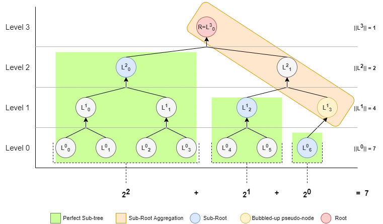
In Fig 1 , every node in the merkle-tree can be addressed by a 2D $ (x,y) $ coordinate. The $ y $-dimension is called the "level" and the $ x $-dimension the "index" at the level. By convention we use $ L^{level}_{index} $ notation. As can be seen, a merkle-tree contains "perfect sub-trees" which are themselves merkle-trees whose leaves are subsets with cardinalities equal to powers of 2.

2.1 Formal definition

For any sequence of $ N $ binary objects $ O=\{O_1, ..., O_{N}\} $ where $ O_i = \{0,1\}^* $ and cryptographic hash function $ \textbf{H}:\{0,1\}^* \rightarrow \{0,1\}^n $, the merkle-tree $ L:(O, x \in \mathbb{Z}_0, y \in \mathbb{Z}_0) \rightarrow \{0,1\}^n $ is defined as the piece-wise chaining-function:

$ L^{y}_{x}(O) = \begin{cases} \textbf{H}(O_{x+1}) &\quad \text{$y=0$ and $0 \le x < N$} &\quad \text{(leaf node)}\\ H(L^{y-1}_{2x}, L^{y-1}_{2x+1}) &\quad \text{$0 < y < h$ and $0 \le x < \frac{\|L^{y-1}\|-1}{2}$} &\quad \text{(parent node)}\\ L^{y-1}_{2x} &\quad \text{$y>0$ and $x = \frac{\|L^{y-1}\|-1}{2}$ and $\|L^{y-1}\| = 1 \pmod{2}$} &\quad \text{(bubble-up node)}\\ \varnothing &\quad \text{otherwise} &\quad \text{(null node)}\\ \end{cases} $

$ \text{where} $

$ \\\\\begin{align*}N &= \|L^0\| = \|O\| &\quad \text{(cardinality of the leaf set)} \\h &= \lceil\log_2N\rceil+1 &\qquad\text{(height of merkle-tree)} \\\|L^n\| &= \left\lceil\frac{N}{2^n}\right\rceil &\qquad \text{(cardinality of level $n$)} \\H(l,r) &= \textbf{H}(l || r) &\qquad\text{(node hash function)}\\\end{align*} $

In this definition, a merkle-tree $ L $ maps a sequence of objects $ O $ and two positive integers $ (x,y) $ to a hash digest $ \{0,1\}^n $. The arguments $ (x,y) $ are the "merkle-coordinates" of a node (digest) in the merkle-tree and are always denoted as super/subscripts of $ L $ (so as to convey their equivalence relation / chaining function nature). However, in this treatment they are strictly arguments of $ L $.

REMARK In this notation, when the argument $ O $ of $ L $ is omitted it shall always be implied. For example the notation $ L^{y-1}_{2x} $ is equivalent to $ L^{y-1}_{2x}(O) $ . The term $ L^y_x $ shall be interpreted as "the node at $ (x,y) $ for the merkle-tree $ L $ of $ O $ ".

2.2 Root

The merkle-root $ R $ is the most fundamentally important node in a merkle-tree and represents a cryptographic hash commitment to the entire tree. Security proofs that verify statements about trees almost always verify to the root.

Definition 2.2.1: Root

The root of a merkle-tree $ L $ with height $ h $ is the node $ R= L^{h-1}_{0} $. QED.

2.3 Descendants

The "descendants" of a node are the set of all transitive child nodes (i.e. child, grand child, great grand-child, etc) up to an until the leaf nodes.

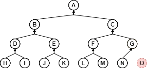
In Fig 2 , the nodes $ B $, $ D $ and $ H $ are the $ 1^{st} $, $ 2^{nd} $ and $ 3^{rd} $ left-most descendants of $ A $ respectfully. On the right side, the nodes $ C $, $ G $ and $ N $ are the $ 1^{st} $, $ 2^{nd} $ and $ 3^{rd} $ right-most descendants of $ A $ respectfully. The non-existent node $ O $ is the $ 3^{rd} $ right-most perfect descendant of $ A $. Had it been a node of the tree, it would also be the right-most descendant (and the tree would be "perfect"). The left-most and right-most leaf-descendant's of $ A $ are $ H $ and $ N $ respectfully. The leaf-descendants of $ A $ are neighbourhood of leaves from $ H $ to $ N $ inclusive.

Lemma 2.3.1: Left-most descendant

For any node $ L^y_x $ the $ k^{th} $ left-most descendant is the node $ L^{y-k}_{2^k x} $ .

Proof: Node $ L^y_x $ has left-child $ L^{y-1}_{2x} $, left-most grand-child $ L^{y-2}_{2(2x)}=L^{y-2}_{2^2x} $ and left-most great grand-child $ L^{y-3}_{2(2(2x))}=L^{y-3}_{2^3x} $. It follows that the $ k^{th} $ left-most child is thus $ L^{y-k}_{2^k x} $ . QED.

Lemma 2.3.2: Right-most perfect descendant

For any node $ L^y_x $ the $ k^{th} $ right-most perfect descendant is the node $ L^{y-k}_{2^k(x + 1) - 1} $ .

Proof: Node $ L^y_x $ has right-child $ L^{y-1}_{2x+1} $, right-most grand-child $ L^{y-2}_{2(2x+1)+1}=L^{y-2}_{2^2x+2^1+2^0} $, right-most great grand-child $ L^{y-3}_{2(2(2x+1)+1)+1}=L^{y-3}_{2(2^2x+2^1+2^0)+1}=L^{y-3}_{2^3x+2^2+2^1+2^0} $. Assuming no bubble-up nodes, it follows the $ k^{th} $ right-most descendant is thus $ L^{y-k}_{2^k(x + 1) - 1} $. QED.

Lemma 2.3.3: Right-most descendant

For any node $ L^y_x $ the $ k^{th} $ right-most descendant is the node $ L^{y-k}_{\min\left(2^k(x + 1), \left\lceil\frac{N}{2^{y-k}}\right\rceil\right) - 1} $ where $ N $ is the leaf count.

Proof: The $ k^{th} $ right-most descendant is either the $ k^{th} $ right-most perfect descendant or the last node at level $ y-k $. It follows from lemma 2.3.2 that in the absence of bubble-up nodes, the $ k^{th} $ right-most descendant index is $ 2^k(x + 1) - 1 $. In the presence of a bubble-up nodes, the index is clipped to the last node at level $ (y-k) $ which, through definition 2.1 , becomes $ \|L^{y-k}\| - 1 = \left\lceil\frac{N}{2^{y-k}}\right\rceil - 1 $ . By taking the $ \min $ of both values, the right-most descendant determined. QED.

Remark 2.3.4

The distinction between a "right-most perfect descendant" and a "right-most descendant" is that the former assumes the descendants are all non-trivial nodes (i.e no bubble-up) whereas the latter does not. For "perfect trees" discussed below, there is no distinction between the two. However, as trees are generally imperfect such a distinction is generally needed. Conceptually, a right-most descendant is the right-most perfect descendant clipped to the end the level (hence the $ \min $ in the equation).

For example, in Fig 2 the nodes $ F $ and $ L $ are the $ 1^{st} $ and $ 2^{nd} $ left-most descendants of $ C $ respectively. On the right-side, $ G $ is the $ 1^{st} $ right-most descendant and $ 1^{st} $ right-most perfect descendant. However, the $ 2^{nd} $ right-most descendant is $ N $ and the right-most perfect descendant does not exist ($ O $). QED.

Theorem 2.3.5: Descendants

The descendants of node $ L^y_x $ is the set is $ D^y_x $ defined as:

$ \begin{align*} D^y_x &= \bigcup_{i=1}^y \left\{L^{y-i}_{j} | j \in \{l, ..., r \} \right\} \\ \text{where}\\ l &= 2^{i}x\\ r &= \min\left(2^i(x + 1), \left\lceil\frac{N}{2^{y-i}}\right\rceil\right) - 1\\ \end{align*} $

Proof: For every level below $ L^y_x $, aggregate via set union the neighbourhood from the left-most to right-most descendent nodes (inclusive) at that level. QED.

Lemma 2.3.6: Leaf descendants

The "leaf-descendants" of $ L^y_x $ is the set $ U^y_x=\{L^0_i | i \in \{l,...,r\}\} $ where:

$ \begin{align*} l &= 2^y x \qquad\qquad\qquad\qquad\qquad\qquad\text{(left-most leaf-descendant)}\\ r' &= 2^y(x + 1) - 1 \qquad\qquad\qquad\qquad\text{(right-most perfect leaf-descendant)} \\ r &= \min\left(2^y(x + 1), \left\lceil\frac{N}{2^{y-k}}\right\rceil\right) - 1 \qquad \text{(right-most leaf-descendant)} \end{align*} $

Proof: The leaf-descendant equations derive from lemmas 2.3.1 - 2.3.3 setting $ k=y $. The leaf-descendants $ U^y_x $ are thus the neighbourhood of nodes from the left-most to right-most leaf descendants (inclusive). QED.

Lemma 2.3.7: Descendant Equality

If a node exists in two trees then so does it's descendants.

Proof: Let $ L^y_x $ and $ I^u_v $ be different nodes in different trees such that $ L^y_x=I^u_v $. It follows from lemma 2.3.6 that $ F^y_x = G^u_v $ where $ F $ and $ G $ are the leaf-descendants of $ L^y_x $ and $ I^u_v $ respectively. QED.

2.4 Powers of 2

Theorem 2.4.1 Powers of 2 Partition

Any number $ N\in\mathbb{Z}_0 $ can be written as a unique sum of the powers of 2 such that $ N = \sum_i 2^{C_i} $ for a set of exponents $ C= \{C_i \in\mathbb{Z}_0\} $ where $ 0 \le \|C\| \le \lceil\log_2 N\rceil $.

Proof: Let $ N = \sum^N_{i=1} 2^0=2^0 + 2^0 + ..\text{N-times} $. This sum contains $ N $ terms. By applying the reduction $ 2^0+2^0=2^{1} $ once the sum reduces to $ N-1 $ terms. By applying the reductions $ 2^k+2^k=2^{k+1} $ for all $ 0 \le k \le \lceil\log_2N\rceil $ repeatedly, the number of terms in the sum converges to $ j $ where $ 0 \le j \le \lceil\log_2N\rceil $. That $ j $ is bound from $ 0 $ follows from the case when $ N=0 $, yielding a sum for $ N $ having no terms. That $ j $ is bound to $ \lceil\log_2N\rceil $ arises from the fact that iteratively dividing any $ N $ by $ 2 $ more than $ \lceil\log_2N\rceil $ times yields no additional terms in the sum. That this is true can be seen from $ \forall N\in \mathbb{Z}, 0=N \div 2^{\lceil\log_2N\rceil + 1} $. Thus the exponents of these $ j $ terms are the set $ C=\{C_1, ..., C_j\} $ where $ j $ is the smallest possible number since no further reductions are possible. Uniqueness is proven by contradiction. Suppose there exists another set of $ j $ irreducible exponents $ C'=\{C'1, ..., C'j\} $ where $ \sum^j{i=1} 2^{C_i} = \sum^j{i=1} 2^{C'_i} $ and $ C' \ne C $. This would imply that $ \exists a\in \mathbb{Z}_0 $ and $ \exists b \in \mathbb{Z}_0 $ such that $ 2^a=2^b \land a \ne b $, an impossibility by virtue of exponentiation being bijective over $ \mathbb{Z}_0 $. Thus $ C $ is unique. QED.

Definition 2.4.2: Pow-2 Partition

The set $ C $ from theorem 2.4.1 is herein coined the "powers of 2 partition of $ N $ " (aka "pow-2 partition") and chosen in descending order. In natural language, the set $ C $ are the exponents of the terms of a partition of $ N $ whose terms are all powers of 2 and, that out of all such partitions, is the one with the least cardinality. The set $ C $ are the exponents of the terms in this partition and chosen by convention in decreasing order. QED.

See table 2.4.7 for examples of pow-2 partitions.

Lemma 2.4.3: Strictly Decreasing

The powers-of-2 partition of $ N $ are a strictly decreasing set $ C $ such that $ C_{i} > C_{i+1} $ for all $ 1 \le i < \|C\| $.

Proof: By definition $ C $ is an ordered decreasing set thus $ C_{i} \ge C_{i+1} $. To be strictly decreasing then $ C_i > C_{i+1} $. If it is assumed that two adjacent exponents where equal such that $ C_{i} = C_{i+1} = x $ then $ 2^{C_i}+2^{C_{i+1}}=2^x+2^x=2^1 2^x=2^{x+1} $. As this is itself a power of 2, one could replace both exponents $ C_i $ , $ C_{i+1} $ with single exponent $ x+1 $ in $ C $. This would necessarily shorten the cardinality of $ C $ thus contradicting the requirement of definition 2.4.2 that it be the partition with least cardinality. Thus since no adjacent exponents in $ C $ can ever equal by virtue of $ C $ being defined as the shortest partition, it follows $ C $ is strictly decreasing. QED.

Algorithm 2.4.5 CalcPow2Partition

Calculates the powers of 2 partition of $ N $. Returns the set $ C $ such that $ N=\sum_{i} 2^{C_i} $ where $ C $ is the partition of least cardinality in decreasing order. Example, for $ N=15 $ the result is $ C=(3,2,1,0) $ since $ 15 = 2^3 + 2^2 + 2^1 + 2^0 $.


 1: algorithm CalcPow2Partition
 2:   INPUT:
 3:      N : Integer
 5:   OUTPUT
 6:      c : array of integer       ; positive integr (0 <= N <= Max)
 7:   PSEUDO-CODE:
 8:      let i = 0
 9:      while ( N >= 1 )
10:         let x = floor(log_2(N))
11:         if x = log_2(N)         ; mantissa is zero
12:            c[i] = x
13:            i = i + 1
14:            N = N - 2^x
15: end algorithm

Algorithm 2.4.6 Reduce

Reduces an arbitrary sum of powers of 2 to an ordered pow-2 partition of the summation. This is the process used in theorem 2.4.1 .


 1: algorithm Reduce
 2:   INPUT:
 3:      N : Array of Integer
 4:   OUTPUT:
 5:      M : Array of Integer
 6:   PSEUDO-CODE:
 7:      let finished = false
 8:      while NOT finished
 9:         for i = Length(N) - 1 to 1
10:            if N[i-1] < N[i]
11:               SWAP N[i-1], N[i]
12:               goto 8
13:            if N[i-1] = N[i]
14:               INCREMENT N[i-1]
15:               N.RemoveAt(i)
16:               goto 8
17:         finished = true
18:      M = N
29: end algorithm

Integers when represented as powers of 2 partitions follow an interesting pattern.

Table 2.4.7 Pow-2 Partitions of N

Integers 0 - 16	Integers 244 - 260	Integers 983-999
0: 1: 0 2: 1 3: 1, 0 4: 2 5: 2, 0 6: 2, 1 7: 2, 1, 0 8: 3 9: 3, 0 10: 3, 1 11: 3, 1, 0 12: 3, 2 13: 3, 2, 0 14: 3, 2, 1 15: 3, 2, 1, 0 16: 4	244: 7, 6, 5, 4, 2 245: 7, 6, 5, 4, 2, 0 246: 7, 6, 5, 4, 2, 1 247: 7, 6, 5, 4, 2, 1, 0 248: 7, 6, 5, 4, 3 249: 7, 6, 5, 4, 3, 0 250: 7, 6, 5, 4, 3, 1 251: 7, 6, 5, 4, 3, 1, 0 252: 7, 6, 5, 4, 3, 2 253: 7, 6, 5, 4, 3, 2, 0 254: 7, 6, 5, 4, 3, 2, 1 255: 7, 6, 5, 4, 3, 2, 1, 0 256: 8 257: 8, 0 258: 8, 1 259: 8, 1, 0 260: 8, 2	983: 9, 8, 7, 6, 4, 2, 1, 0 984: 9, 8, 7, 6, 4, 3 985: 9, 8, 7, 6, 4, 3, 0 986: 9, 8, 7, 6, 4, 3, 1 987: 9, 8, 7, 6, 4, 3, 1, 0 988: 9, 8, 7, 6, 4, 3, 2 989: 9, 8, 7, 6, 4, 3, 2, 0 990: 9, 8, 7, 6, 4, 3, 2, 1 991: 9, 8, 7, 6, 4, 3, 2, 1, 0 992: 9, 8, 7, 6, 5 993: 9, 8, 7, 6, 5, 0 994: 9, 8, 7, 6, 5, 1 995: 9, 8, 7, 6, 5, 1, 0 996: 9, 8, 7, 6, 5, 2 997: 9, 8, 7, 6, 5, 2, 0 998: 9, 8, 7, 6, 5, 2, 1 999: 9, 8, 7, 6, 5, 2, 1, 0

The $ \text{reduce} $ algorithm allows integer arithmetic to be expressed purely in terms of increments, bit-shifts, comparisons and memory read/writes. It is the opinion of the author that this construction is significant (but unsure if necessarily novel). For one, it greatly simplifies Big Integer implementations by reducing their representations to pow-2 partition forms. Big Integer arithmetic simplifies to primitive set transformations and a some iterations of the $ \text{reduce} $ function. For example, two add two numbers one need only $ \text{reduce} $ the concatenation of their pow-2 partitions, as shown by theorem theorem 2.4.8 . Similarly to multiply two integers, one need only $ \text{reduce} $ the cartesian product of the pow-2 partitions, as shown by theorem 2.4.9 . With these two approaches, a Big Integer implementation (properly implemented) ought to improve performance significantly compared to existing implementations. This follows by virtue of not requiring any underlying string manipulations or aggregation of smaller integer arithmetic. Also, from a fundamental number theory point of view, a description of arithmetic in terms if more primitive operations illuminates insight into the nature of numbers themselves.

Theorem 2.4.8: Integer Addition in terms of Reduce

For all $ a \in \mathbb{Z}_0 $ and $ b \in \mathbb{Z}_0 $, if $ c = a + b $ then $ C = \text{reduce}(A || B) $ where $ A, B, C $ are the pow-2 partitions of $ a, b, c $ respectfully.

Proof: Start with $ a=\sum_i 2^{A_i} $ and $ b=\sum_i 2^{B_i} $ . It follows that $ a + b =\sum_i 2^{A_i} + \sum_i 2^{B_i} = \sum_i 2^{G_i} $ where $G = A || B$ . Here $ G $ represents the concatenation of $ A $ and $ B $ and gives a sequence of exponents such that $ c=\sum_i2^{G_i} $. To recover $ C $, the sequence $ G $ is reduced to pow-2 partition form through $ C=\text{reduce}(G) $. QED.

Theorem 2.4.9: Integer Multiplication in terms of Reduce

For all $ a \in \mathbb{Z}_0 $ and $ b \in \mathbb{Z}_0 $, if $ c = ab $ then $ C = \text{reduce}(A \times B) $ where $ A, B, C $ are the pow-2 partitions of $ a, b, c $ respectfully and $ A \times B = \{u+v:u \in A \land v \in B\} $ denotes a cartesian product taking the sum of the pairs.

Proof: Start with $ a=\sum_i 2^{A_i} $ and $ b=\sum_i 2^{B_i} $ . It follows $ ab =\sum_i 2^{A_i} \sum_i 2^{B_i}=(2^{A_1} + 2^{A_2} + ...+2^{A_n})(2^{B_1} + 2^{B_2} + ...+2^{B_m}) $. Through distributive and exponent law, $ ab=(2^{A_1+ B_1} + 2^{A_1+B_2} + ... +2^{A_2 + B_1} + 2^{A_2 + B_2} + ... +2^{A_n+B_m})=\sum_i 2^{G_i}=c $ where $ G = A \times B $ . Here $ G $ represents the cartesian product taking the sum of the pairs. To recover $ C $, the sequence $ G $ is reduced to pow-2 partition form through $ C=\text{reduce}(G) $. QED.

2.5 Perfect Trees

A interesting characteristic of merkle-trees is their relationship to what are hereby coined "perfect trees".

Definition 2.5.1: Perfect tree

A perfect-tree is a merkle-tree having $ N $ leaves and height $ h $ such that $ N=2^h $. QED.

Perfect trees have special properties as illustrated by Fig 1 . By inspection alone, one can see that generally imperfect merkle-trees are composed from perfect sub-trees whose roots can be aggregated to determine the merkle-root. Also, it's clear that perfect sub-trees remain invariant after leaves are appended to the tree. That a merkle-tree is in fact such an aggregation of such perfect sub-trees is shown in theorem 2.6.3 .

Lemma 2.5.2: Perfect sub-trees

A merkle-tree $ L $ with $ N $ contains an ordered set of perfect sub-trees $ P=\{P_1,..,P_{\|C\|}\} $ where $ C $ is the pow-2 partition of $ N $ and the height of $ P_i=C_i $.

Proof: For every exponent $ C_i $ construct a perfect tree $ P_i $ having $ 2^{C_i} $ leaves, let this set of perfect trees be $ P=\{P_1,..,P_j\} $. Choosing the leaves of $ P_i $ as $ \{L^{0}{x},...,L^{0}{x+2^{C_i}-1}\} $ where $ x = \sum_{k=1}^{i-1} 2^{C_k} $ maps all leaves of $ L $ via bijection to the union of all the leaves in $ P $. Through lemma 2.3.7 it follows that the antecedents of the union of the leaves in $ P $ are contained within $ L $. Thus all nodes in $ P $ are fully contained in $ L $, in order, noting that only the imperfect bubble-up nodes of $ L $ are not in any of $ P $. QED.

Lemma 2.5.3: Perfect Nodes

A merkle-tree $ L $ with $ N $ leaves has $ \sum_i (2^{C_i} - 1) $ perfect nodes where $ C $ is the pow-2 partition of $ N $.

Proof: A perfect tree $ P $ of height $ h_P $ with $ N_P $ leaves has total $ 2^{h_P} - 1 $ nodes. This follows from the relation $ \sum^{n-1}{i=0} 2^i=2^n-1 $. The sum on the left is aggregates the level count for each perfect tree. As per lemma 2.5.2 , a merkle-tree is composed of perfect-trees $ P=\{P_1,..,P{\|C\|}\} $ where the height of $ P_i = C_i $. Thus by summing the node count for all $ P_i $ we get $ \sum_i (2^{C_i} - 1) $ which are the count of all the perfect nodes in $ L $. QED.

2.6 Sub-Roots

An important aspect of perfect sub-trees is the role their roots play in the larger imperfect parent tree. The roots of perfect sub-trees are herein called the "sub-roots" of the parent tree and have special properties that are used in security proofs, particularly in append-proofs which prove a leaves were appended by transformation of the sub-roots alone.

Lemma 2.6.1: Sub-Roots

The sub-roots $ S $ of a merkle-tree $ L $ with $ N $ leaves are the nodes $ S = \left\{(P_i)^{C_i}_{0} | 1 \le i \le \|C\|\right\} $ where $ P $ are the perfect sub-trees of $ L $ and $ C $ the exponents of the powers-of-2 partition of $ N $.

Proof: $ S $ is the set of merkle-roots for all $ P_k \in P $. The merkle-root of $ P_k $ is found at $ y $-coordinate $ C_i $ and $ x $-coordinate $ 0 $ on tree $ P $. QED.

The blue nodes in Fig 1 illustrate the sub-roots and how their values directly aggregate to merkle-root. This aggregation chain is depicted by the orange rectangle and comprised of nodes which are bubbled-up sub-roots. Since this orange rectangle appears for every imperfect tree, it suggests that the merkle-root can be calculated directly from the sub-roots. Indeed this is proven in by theorem 2.6.3 and implemented by algorithm 2.6.4 .

Lemma 2.6.2: Sub-Root Invariance

A sub-root $ L^y_x $ of a merkle-tree $ L $ with $ M $ leaves remains invariant after a leaf-append transformation to $ N \ge M $ leaves.

Proof: This follows from remark 2.3.4 in that since the $ L^y_x $ is a sub-root, it is a perfect node and it's right-most leaf-descendant $ L^0_{2^y(x + 1) - 1} $ must exist in the pre-transformation tree. Since the post-transformation tree only appends leaves after $ 2^y(x+1)-1 $, it necessarily implies the leaf descendants of $ L^y_x $ remain unaltered. Thus by lemma 2.3.7 , so do all antecedent nodes. QED.

Remark 2.6.3

Lemma 2.6.2 does not suggest $ L^i_j $ remains a sub-root in the post-transformation tree, only that it's value remains invariant.

Theorem 2.6.3: Sub-Root Aggregation

If $ S $ are the sub-roots of a merkle-tree $ L $ then the merkle-root $ R $ can be calculated as $ R=Aggr(S,\|S\|) $ where $ Aggr:(\{\{0,1\}^n\}^*, \mathbb{N}) \rightarrow \{0,1\}^n $ is a chaining function defined as:

$ \begin{align*} Aggr(S,i) &=\begin{cases} S_{\|S\|} &\quad\text{$i=1$} \\ H^{\top}(Aggr(S,i-1), S_{\|S\|-i+1}) &\quad \text{otherwise} \end{cases} \\ \text{where} \\ H^{\top}(l,r) &= H(r,l) \qquad \qquad \qquad \qquad \qquad \quad \quad \text{(transposed node hash)} \end{align*} $

See Algorithm 2.6.4: Aggregate Roots for a simple implementation of $ Aggr $.

Proof: First it is shown that the sub-roots alone are sufficient to compute the root. This follows from the fact that the union of all the leaf descendants of the sub-roots encumber all the non-trivial nodes of the tree except the sub-roots (and bubble-up's of the sub-roots). Another way is by contradiction, since if some node $ k $ not a sub-root were also required to calculate $ R $ then the hash-chain of $ R $ would necessarily include $ k $ twice violating definition 2.1 . This follows since $ k $ being a descendant of a sub-root $ S_i $, would appear twice in the hash-chain of $ R $ first as a part of $ S_i $'s sub-chain and independently. Therefore, let $ T:\{\{0,1\}^n\}^* \rightarrow \{0,1\}^n $ be mapping from the sub-roots $ S $ to the root $ R $ such that $ R=T(S) $. In the case where only a single sub-root exists $ S=\{S_1\} $ and the is $ R=S_1 $, thus $ T(S)=S_1=R $. For the case when $ \|S\|>1 $, using definition 2.1 of a parent node we derive $ R=H(S_n,H(...,H(S_d,H(S_c,H(S_b,S_a))))=T(S) $ for some ordering $ (a,b,c,...,n) $. In other words, it is a hash-chain of the sub-roots in an explicit ordering. To determine this ordering, we observe that the sub-roots $ S $ map along coordinates of $ L $ in a strictly decreasing manner from left to right, top to down. That this is so follows from the fact that the levels of the sub-roots of $ L $ are a bijection to the pow-2 partition of the leaf count of $ L $, a strictly decreasing sequence lemma 2.4.3 . Therefore, the right-most sub-root is the lowest in the tree, the second right-most is the second lowest, et al. Since hash-chains start from the leaf level, it follows that the lowest sub-root is first in the hash-chain, the second lowest is second, et al. We thus solve $ (a,b,c,..., n) = (n, n-1, n-2, ..., 1) $. Plugging back into $ R $ gives $ R=H(S_1,H(S_2,H(S_3, H(...,H(S_{n-1}, S_n))))) $. Rewriting using transposed node-hasher $ H^{\top} $ gives $ R=H^{\top}(H^{\top}(H^{\top}(H^{\top}(S_n, S_{n-1})..., S_3),S_2),S_1)=T(S) $. Finally, observe that $ Aggr $ is the function $ T $ parameterized by $ i $, an index into the hash chain. Thus it follows that the $ R $ would be the last index in that chain, hence $ R=Aggr(S, \|S\|) $. QED.

Algorithm 2.6.4: Aggregate Roots

Calculates the merkle-root from the sub-roots as per theorem 2.6.3 .


 1: algorithm CalcRoot
 2:   INPUT:
 3:      S : array of digest           ; sub-roots
 4:   OUTPUT:
 5:      Result : digest
 6:   PSEUDO-CODE:
 7:      Result = S[^1]                ; ^1 is last index
 8:      for i = Length(s) - 2 to 0    ; start from second last
 9:         Result = H(S[i], Result)   ; transposed H^T(l,r) = H(r,l)
10: end algorithm

2.7 Node Traversal

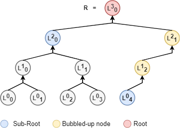
Most merkle-trees are imperfect and will contain at least one bubble-up node. In the Fig 3 below, the leaf node $ L^0_4 $ bubbles up to become the root $ R $'s right-child. In proof constructions, these bubble-up paths are, for the most part, implicitly traversed. In order to distinguish between traversal or not, the following terminology is employed: "logical left-child", "logical right-child", "logical sibling" and "logical parent". In this context, "a logical relationship" denotes that the bubble-up path is implicitly traversed until the first non-bubbled up node is encountered. For example, in Fig 3 the sibling of $ L^2_0 $ is $ L^2_1 $ but the logical sibling is $ L^0_4 $. The right-child of $ L^3_0 $ is $ L^2_1 $ but the logical right-child is $ L^0_4 $. Similarly, the logical left-child of $ L^2_1 $ is $ L^0_4 $ and the logical parent of $ L^0_4 $, $ L^1_2 $ and $ L^2_1 $ is $ L^3_0 $.

3. Security Proofs

A system of formal security proofs is presented here which permits a verifier, knowing only the merkle-root, to verify membership of the tree and explicit transformations of the tree to new merkle-roots. This allows a verifier to track the evolution of a merkle-tree without the burden of storing such tree yet maintaining a commensurate level of security (bound by underlying cryptographic hash function). In other words, they can track a dynamic merkle-tree.

Such a proof system is desirable for applications where maintaining merkle-trees is computationally and/or storage-wise expensive. Such applications include blockchain applications and decentralized ledger technologies in general. Through these algorithms consensus systems can be made to scale for real-time, global adoption with near 0 storage and computational complexity.

Number	Proof Name	Description
3.2	Existence	Proof a node exists within a tree
3.3	Ranged Existence	Proof a subset of leaves* exists within a tree
3.4	Right Delete (Consistency)	Proof that leaves were deleted from right of a tree
3.5	Append	Proof that leaves were appended to the right of a tree
3.6	Remove	Proof a count of leaves from removed from the right of a tree
3.7	Update	Proof that a single node was updated within a tree
3.8	Ranged Update	Proof that a subset of leaves* were updated within a tree
3.9	Insert	Proof that a neighbourhood of leaves were inserted arbitrarily within a tree
3.10	Delete	Proof that a neighbourhood of leaves were deleted arbitrarily from a tree
3.11	Subset	Proof that a neighbourhood of leaves** exists within a tree
3.12	Substitution	Proof that a neighbourhood of leaves** was substituted 1 - 1, within a tree

*: not necessarily contiguous

**:without specifying leaves

3.1 Proof Construction

A security proof consists of start digest $ D_0 $, a set of digests $ D=\{D_1, ... D_n\} $, a set of direction flags $ F=\{F_1, ..., F_n\} $ and a root-digest $ R $. To verify the proof, the verifier must hash of the set of digests $ D $ in a chain using a cryptographic node-hash function $ H(l,r) $ and starting with $ D_0 $. In each step of the aggregation, the ordering of the arguments in $ H $ is determined by the corresponding flag in $ F $. See reference implementation [2] for specification and Fig 3 for an example .

3.2 Existence

An existence proof is a proof that a node exists within a tree. Specifically, it is a proof that the node $ L^y_x $ has value $ z $ for a tree $ L $ with root $ R $. Existence proofs are generally used to prove the existence of leaf nodes. However, in this paper, they are also used to prove the existence of sub-roots which can be anywhere in the tree. This algorithm is well-known in the literature as an "audit proof", and provided here for brevity.

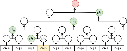
The existence-proof for $ \text{Obj 3} $ comprises of the hash-path $ D=\{L^0_2, L^1_0, L^2_1, L^3_1\} $ and the object $ \text{Obj 3} $ and the index $ i=3 $ of the object. The verifier has the merkle-root $ R $ and knows the total leaf-count $ N=9 $. Knowing the index $ i $, the verifier computes the direction flags $ F=\{0, 0, 1, 1\} $ which represent which side of the hash-function a node's digest is an argument of. The verifier then computes the start digest $ D_0=L^0_3 $ by hashing $ \text{Obj 3} $. The verifier then performs $ R' = H(H(H(D_2, H(D_1, D_0)), D_3), D_4) $ noting that the ordering of the hash arguments $ D_i $ is determined by flag $ F_i $. The verifier knows if $ R'=R $ then proof is valid and $ \text{Obj 3} $ exists at index $ i=3 $, otherwise it is invalid.

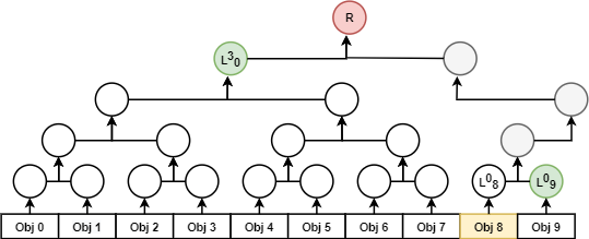
Similarly, the existence-proof for object 8 comprises of start digest $ D_0=L^0_8 $, hash-path $ D=\{L^0_9, L^3_0\} $, flags $ F=\{1, 0\} $ and root $ R $. The verifier checks that $ R=H(D_2, H(D_0, D_1)) $. Of note in Fig 4 is the implicit traversal of bubble-nodes by virtue of the logical parent/siblings algorithms found the reference implementation [2] .

3.3 Ranged Existence

A ranged-existence-proof extends an existence-proof to multiple leaf nodes (not necessarily adjacent). The purpose is to provide $ 1 $ proof that $ N $ leaves exist rather that relying on $ N $ proofs that $ 1 $ leaf exists. Since neighbouring leaf nodes tend to share antecedent nodes, by taking the union of all their individual existence-proof paths a significant saving in space complexity is achieved. See reference implementation [2] for specification.

3.4 Right Delete (Consistency)

A consistency-proof proves that the first $ M $ leaves of two trees are equal. In other words, it proves that a merkle-tree $ L $ with $ M $ leaves and root $ R $ has the same first $ M $ leaves as tree $ L' $ with $ N \ge M $ leaves and root $ R' $. The consistency-proof construction in this paper is unique and differs from commonly known implementations. In the opinion of the author, the construction here is more elegant and simpler. It works by proving that the invariant right-most sub-root $ k $ of the smaller tree $ L $ exists in the larger tree $ L' $. If the trees are consistent to $ M $ leaves, the existence-proof of $ k $ in $ L' $ necessarily traverses the existence-path of $ k $ in $ L $. This allows $ R $ to be recovered from the existence-proof of $ k $ in $ L' $ alone. By verifying $ R $ indeed derives from the existence-proof of $ k $ in $ L $, and the existence proof itself validates to $ R' $, then the verifier shown $ L $ and $ L' $ are consistent up to and including $ M $ leaves. See reference implementation [2] for specification.

REMARK 3.4.1: In other treatments, consistency proofs are proffered as a (weak) proof that a tree was appended to with new leaves. In the opinion of the author, consistency-proofs are a weak form of proving an append since they only prove that a count of leaves were appended but say nothing about the appended leaves themselves. In practice, knowing that items were appended to a list but without knowing what those items were can lead to insecure assumptions about the system. A consistency-proof only proves the post-transformation leaf-set of a tree is consistent with the pre-transformation leaf-set and nothing more. With this in mind, it is the opinion of the author that a "consistency proof" ought to be correctly interpreted as a "right-delete-proof" in reverse. In other words, a right-delete-proof proves that a tree $ L' $ with $ N $ leaves and root $ R' $ becomes a tree $ L $ with $ M<=N $ leaves with root $ R $. This is equivalent to a consistency proof in reverse but is "strong" in the sense that it completely proves the "right-deletion" (rather than "weakly" proves an append). By preference to elegancy, the primary form of this proof ought be a right-delete-proof and a consistency-proof ought to be considered a delete-proof in reverse. However, to maintain parity with existing convention, we treat a "right-delete-proof" as a reverse of a "consistency-proof".

3.5 Append

An append-proof is a new type of security proof that permits a verifier to prove, knowing only the merkle-root, that a specific subset of leaves were appended to a merkle-tree. In this scenario, the verifier is assumed to have the appended leaves $ A=\{A_1, ..., A_n\} $ and the merkle-root $ R $ of the pre-appended tree. Given an append-proof $ P $, the following construction permits the verifier to compute the post-append merkle-root $ R' $ using only $ R $, $ A $ and $ P $.

The proof $ P $ is simply the sub-roots $ S $ of the pre-append tree (a surprisingly small set). For example, if $ N $ is the leaf count then $ 0 <= \|P\| <= \lceil\log_2N\rceil $. The verifier proceeds by iteratively transforming $ S $ with every item in $ A $ in accordance with append leaf algorithm 3.5.1 . The transformed sub-roots $ S' $ are then aggregated via algorithm 2.6.4 to recover $ R' $. In this manner, the verifier proves that the only change to the leaves of $ R $ was the right-append of $ A $, resulting in $ R' $.

The space and time complexity of this proof is $ O(\frac{1}{2}\log_2(N) +\|A\|) $. The $ \frac{1}{2}\log_2N $ term derives as the average cardinality of the sub-roots of $ N $ for increasing $ N $, and $ \|A\| $ self-evidently denotes the count of items being appended. When appending small sets of leaves to large trees (i.e. $ N >> A $) the space and time complexity becomes $ O(\frac{1}{2}\log_2(N)) $. This is the primary use-case for this proof. In the opinion of the author, this new security proof construction offers a significant innovation in the area of merkle-trees. Algorithm 2.6.4 is modelled after a $ \text{reduce}(\phi(N) || \phi(1)) $ where $ \phi $ maps an integer argument to it's pow-2 partition. Conceptually it is "adding $ 1 $ to $ N $ " but in a "hash-based arithmetic". In other words, the algorithm transforms the sub-roots as if they were a pow-2 partition being incremented by $ 1 $ (replacing exponentiation with hashing). This algorithm is also the basis for a spatially-optimized merkle-tree implementation suitable for the efficient construction of practically unbounded trees.

Algorithm 3.5.1 Append Leaf

Transforms a tree's sub-roots $ S $ by appending $ L $ to the leaf set of the tree.


 1: algorithm AddLeaf
 2:   INPUT:
 3:      S : Array of 2-Tuple (Height : Integer, Digest : Integer)
 4:      L : Digest
 5:   OUTPUT
 6:      S : Array of 2-tuple (Height : Integer, Digest : Integer)
 7:   PSEUDO-CODE:
 8:      let e = 2-Tuple (0, L);
 9:      while (true)
10:         if (||S|| = 0 || S[^-1].Height > e.Height)  ;^-1 is last index
11:            S.Add(e)
12:            break while;
13:         e = (S[^1].Height + 1, H(S[^1].Digest, e.Digest))
14:         S.RemoveAt(^1)
15: end algorithm

3.6 Remove

A remove-proof allows a verifier to prove that specific leaves were removed from the right of a tree. It achieves this by simply by re-interpreting an append-proof in reverse by virtue of it's symmetry. In more formal terms, proving that a tree with root $ R' $ and leaf count $ N $ attained the root $ R $ and leaf count $ M=N-\|A\| $ after removing leaves $ A $ from the right is equivalent to an append-proof that a tree with root $ R $ and leaf count $ M $ attained the root $ R' $ and leaf count $ N=M+\|A\| $ after appending $ A $ to the right. Thus a remove-proof is an append-proof in reverse.

3.7 Update

An update proof is a new type of security proof that permits a verifier to prove, knowing only the merkle-root $ R $, that a single node $ k $ was updated to $ k' $ resulting in a new root $ R' $. The update proof comprises simply of an existence-proof of $ k $ in $ R $ denoted $ P $, bundled with $ k $ and $ k' $. Having the root $ R $, the verifier first confirms $ k $ exists in $ R $ by running $ P $ using the start-digest $ k $. Once confirmed, the verifier re-runs $ P $ using start-digest $ k' $ to recover the new root $ R' $.

3.8 Ranged Update

A ranged-update-proof extends an update-proof in much the same way that a ranged-existence-proof extends an existence-proof. It provides a single proof that $ N $ leaves were updated which is far more space and time efficient than $ N $ proofs of $ 1 $ leaf update. This construction comprises of a ranged-existence-proof of the old leaf values coupled with the old leaf values themselves. The verifier first runs an existence-proof of the old leaf values to ensure the root old $ R $ is recovered. The verifier then maps the digests in the proof to their corresponding nodes in a partial merkle-tree, by calculating the path of that proof. It then proceeds to iteratively update the tree for every new appended leaf value. It concludes by verifying that the root of the updated tree matches the expected new root. If it does, it proves that the only change from $ R $ to $ R' $ was the update of the leaves. This construction is provided in the reference implementation [2] .

3.9 Insert

An insert-proof is a general proof of insertion into the tree leaf-set. This is a high-level proof composed of base proofs 3.2 - 3.5 . it proves that the neighbourhood of leaves $ I $ are inserted after $ A $ and before $ B $.

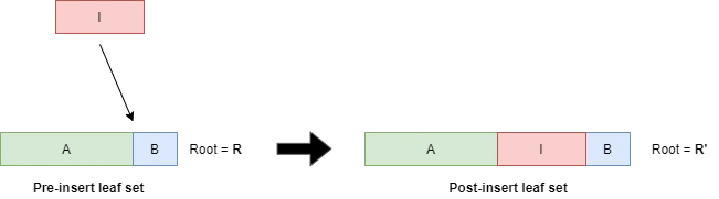
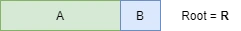
Proving that a tree with root $ R $ had leaves $ I $ inserted after $ A $ and before $ B $ resulting in root $ R' $ is constructed as follows:

A ranged-existence-proof of $ B $ in $ R $.
A right-delete proof of $ \|B\| $ leaves from $ R $ resulting in root $ R_1 $.
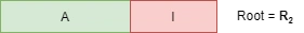
An append-proof of leaves $ I $ to $ R_1 $ resulting root $ R_2 $.
An append-proof of $ B $ to $ R_2 $ resulting in $ R' $.

In practice, an insert proof would be implemented as an ordered sequence of the sub-proofs. A verifier would evaluate the proof by evaluating the sub-proofs in order, ensuring each step verifies to the root that was the output of the preceding step (the first step verifies to to start root).

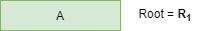
3.10 Delete

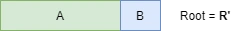
A delete-proof is a general proof of deletion from the tree leaf-set. Specifically, it proves that a neighbourhood of leaves $ D $ after $ A $ and before $ B $ was removed.

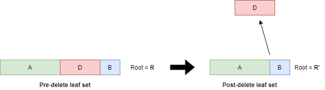
Proving that a tree with root $ R $ had leaf neighbourhood $ D $ removed resulting in the neighbourhood $ A $ joined to neighbourhood $ B $ as follows from:

A ranged-existence-proof of $ B $ in $ R $.
A right-delete proof of $ \|B\|+\|D\| $ leaves from $ R $ resulting in root $ R_1 $.
An append-proof of $ B $ to $ R_1 $ resulting root $ R' $.

3.11 Subset

A subset-proof is a proof that a neighbourhood of leaves in one tree exist in another. Whilst similar in principle to a ranged-existence proof, a subset proof makes no statement about individual leaves in the neighbourhood, only about the neighbourhood itself. A trivial example of a subset-proof is a merkle-root comparison. If two trees share the same root then they share the same leaves (and all other nodes). We extend this concept for all perfect nodes in a tree. By showing the existence of such a node in both trees, it necessarily implies the existence of all their leaf descendants in both trees (by virtue of lemma 2.3.6 ).

Subset proofs only work for leaf-descendants of perfect-nodes which is generally restrictive. As a result, a subset proof is a special-case security proof with a limited domain of applicability. To construct this proof, consider two trees $ L $ and $ K $ sharing a common leaf subset $ S=\{L^0_u, ..., L^0_v\}=\{K^0_{u'}, ..., K^0_{v'}\} $. The prover must find the antecedent node $ p=L^y_x $ such that the left-most and right-most leaf descendant indices are $ u $ and $ v $ respectfully. Similarly for the other tree, the provider finds antecedent $ p'=K^{y'}_{x'} $ for left/right leaf descendants $ u' $ and $ v' $. Use lemma 2.3.6 to get $ u=2^y x $, $ v=2^y(x+1)-1 $ and $ u'=2^{y'} x' $ and $ v'=2^{y'}(x'+1) -1 $. Assuming $ p $ and $ p' $ can be solved, the prover sends both their existence-proofs of $ p $ and $ p' $ coupled with digest of $ p $, to the verifier.

The verifier proceeds to verify the existence of $ p $ in $ L $ and $ p' $ in $ K $ by assuming $ p' $=$ p $. If both both proofs pass then it has been proven that $ S $ exists in both trees and their respective offsets.

REMARK 3.11.1: Due to the requirement that $ S $ be the leaf descendants of a perfect-node, it greatly restricts the possible sets $ S $ applicable for this proof due to odd index numbers and neighbourhoods overlapping subtree leaf-boundaries. Furthermore, when $ S $ is in a different location in $ K $, the restriction exacerbates by applying twice (once per tree). Any attempt to split the neighbourhood $ S $ into acceptable sub-neighbourhoods rapidly converges to $ \|S\| $ splits, one per node. Thus such attempts are equivalent to a ranged-existence proof.

3.12 Substitution

Following from subset-proof , a substitution proof is a proof that a neighbourhood of leaves $ S $ was replaced by another neighbourhood $ S' $ (of equal magnitude) with all other leaf nodes remaining invariant. This is similar in construction to the subset-proof but simpler in that the prover only solves for antecedent node $ p $ of the neighbourhood $ S $ once, and just sends the existence proof of $ p $ in $ L $ to the verifier (along with the old and new digest values for $ p $ and $ p' $). The old value $ p $ denotes the commitment to the old neighbourhood $ S $ whereas $ p' $ a commitment to neighbourhood $ S' $. The verifier begins by validating the existence of $ p $ in $ L $ and then re-running the proof using $ p' $. If the result matches the post-transformation root $ R' $, the proof has shown that $ S' $ replaces $ S $ in $ L $.

REMARK 3.12.1 Like subset-proof, the substitution-proof suffers from limited domain of applicability. However, since only one tree is involved it less severe thus could find utility in specialized cryptographic constructions and consensus workflows.

4. Tree Implementations

This section discusses merkle-tree implementations of relevance. A "flat-tree" is described which permits efficient storage of a tree as a single contiguous block of memory. Appending or right-deleting leaves grow and shrink the memory buffer without invalidating other nodes. In addition, a merkle-tree implementation called "long trees" is discussed which permit unboundedly large tree construction with negligible storage.

4.1 Flat Coordinates

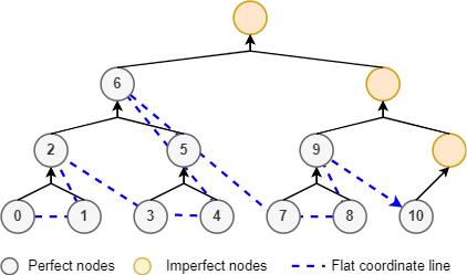
In this section, a system of merkle-coordinates is constructed that flatten the $ (x,y) $ 2-tuple into a single positive integer value $ z \in \mathbb{Z}_0 $. The purpose of these flat coordinate addressing is to permit storage of a dynamic merkle-tree in contiguous memory. In other words, as new nodes are appended to the tree the node buffer can be expanded without affecting prior node values, and similarly when shrinking.

The flat-coordinate line traces out the tree nodes in an interesting diagonal "wave" pattern emanating from $ 0 $ and covering the perfect nodes in ordered sequence. This ordered set of nodes is coined the "ordinal nodes" of the tree. Imperfect nodes are not traced by flat coordinates as they are transient by nature and thus subject to change with the tree as it is appended (unlike ordinal nodes) . As a result, imperfect nodes must be computed on-the-fly. Flat coordinates solve the memory fragmentation problem when dealing with large trees. Due to their high node count, allocating each node separately can lead to excessive memory fragmentation which exhausts memory by future preventing allocations. This can lead to out-of-memory issues despite such memory being available.

The coordinate projection from merkle-coordinates to flat coordinates is a function $ F : (\mathbb{Z}_0,\mathbb{Z}_0) \rightarrow \mathbb{Z}_0 $ and described by algorithm 4.1.2 . Similarly, the inverse projection from flat coordinates to merkle-coordinates $ F^{-1} : \mathbb{Z}_0 \rightarrow (\mathbb{Z}_0,\mathbb{Z}_0) $ is described by algorithm 4.1.3 .

Refer to the following C# algorithms for algorithm implementations:

Algorithm 4.1.2 To Flat Index


public static ulong ToFlatIndex(MerkleCoordinate coordinate) {
	// Step 1: Find the closest perfect root ancestor
	var numNodesBefore = (1UL << coordinate.Level + 1) * ((ulong)coordinate.Index + 1) - 1;
	var rootLevel = Array.BinarySearch(PerfectLeftMostIndices, numNodesBefore);
	if (rootLevel < 0)
		rootLevel = ~rootLevel;
	var perfectRoot = MerkleCoordinate.From(rootLevel, 0);
	Debug.Assert(perfectRoot.Level >= coordinate.Level);

	// Step 2: calculate the path to root, tracking left/right turns
	var flags = new int[perfectRoot.Level - coordinate.Level];
	for (var i = 0; i < flags.Length; i++) {
		flags[i] = coordinate.Index % 2;
		coordinate = MerkleCoordinate.From(coordinate.Level + 1, coordinate.Index / 2);
	}

	// Step 2: Traverse from root down to the node, adjusting the flat index along the way
	var flatIX = PerfectLeftMostIndices[rootLevel];
	for (var i = 0; i < flags.Length; i++) {
		if (flags[flags.Length - i - 1] == 0)
			// moving to left child, so flat index decreases by the difference between the corresponding roots.
			flatIX -= PerfectLeftMostIndices[rootLevel - i] - PerfectLeftMostIndices[rootLevel - i - 1];
		else
			flatIX--;  // moving to right child, so flat index decreases by one
	}
	return flatIX - 1;  // decrease by one, since 0-based indexing
}

Algorithm 4.1.3 From Flat Index


MerkleCoordinate FromFlatIndex(ulong flatIndex) {
	flatIndex++; // algorithm below based on 1-based indexing
	var rootLevel = Array.BinarySearch(PerfectLeftMostIndices, flatIndex);
	if (rootLevel < 0)
		rootLevel = ~rootLevel; // didn't find, so take next larger index

	var index = 0;
	var rootFlatIX = PerfectLeftMostIndices[rootLevel];
	while (flatIndex != rootFlatIX) {
		var isRight = flatIndex > rootFlatIX >> 1;
		index = 2 * index + (isRight ? 1 : 0);
		rootFlatIX = PerfectLeftMostIndices[--rootLevel];
		if (isRight)
			flatIndex -= rootFlatIX;
	}
	return MerkleCoordinate.From(rootLevel, index);
}

Noting that,


PerfectLeftMostIndices = new ulong[63];
for (var i = 1; i < 64; i++) {
	PerfectLeftMostIndices[i - 1] = (1UL << i) - 1;
}

Definition 4.1.4 Ordinal Nodes

The ordinal nodes of a merkle-tree $ L $ are the set $ E=\{F(i) | \forall i \in Z_0 \land 0 \le i < W \} $ where $ F $ is algorithm 4.1.3 and $ W $ the cardinality of the ordinal nodes.

Lemma 4.1.5 Cardinality of Ordinal Nodes

For merkle-tree $ L $ with leaf-count $ N $, the cardinality of the ordinal nodes of $ L $ is $ W=\sum_i (2^{C_i} - 1) $ where $ C $ is the pow-2 partition of $ N $.

Proof: This follows directly from Lemma 2.5.3: Perfect Nodes .

4.2 Long Trees

A long-tree is a specialized merkle-tree suitable for tracking an unbounded lists of objects in $ O(\frac{1}{2}\log_2N) $ space and time complexity. Long merkle-trees are suitable for use-cases where very large trees need to be constructed rapidly and/or maintained indefinitely. These mutations occur through append-only operations (although not strictly required). Example use-cases for these trees include efficient "big block" construction in blockchain consensus systems as well as high-frequency blockchains.

Under the hood, long-trees only maintain the sub-roots of the tree and nothing else. When appending a leaf node the sub-roots are mutated in accordance with algorithm 3.5.1 . Long-trees can only be mutated intrinsically through leaf append transformations. By this we mean that by knowing only the sub-roots it's only possible to append to the tree, not delete, insert, etc. However, through the use of security proofs constructed by fuller tree implementations (such as flat-trees), the tree can be mutated arbitrarily. To achieve this, the security proofs should never refer to merkle-roots directly but always to their sub-roots. The merkle-root can be easily calculated from the sub-roots when needed, however the sub-roots can never be recovered from the root. Thus a system of proofs that bundles the sub-roots in place of roots allows a long-tree to adopt those sub-roots after verifying the proofs. It's important to note that whilst long-trees can mutate arbitrarily through security proofs, the proofs themselves must be constructed by trees that maintain fuller node sets. Thus a consensus network could not comprise exclusively of long-tree nodes. They necessarily require nodes which maintain the full tree (such as flat-trees) in order to construct the general mutation proofs which can be verified by long-tree peers. The reader is referred to the reference implementation[4] for specification.

Remark 4.2.1 A hybrid implementation of long-tree that tracks a neighbourhood of leaves (the last $ M $ leaves) would allow all the peers in P2P consensus network to verify and construct a full set of dynamic merkle-proofs for that neighbourhood. With this approach, peers in P2P consensus network can be comprised of peers that all use a hybrid long-tree implementation. Use-cases here include "deletable blockchains" with checkpoints. The the view of author, long-trees are a significant innovation in the field of merkle-trees.

4.3 Flat Trees

A flat tree is a merkle-tree implemented under the hood using flat coordinates . A flat-tree tracks all it's ordinal nodes in a contiguous block of memory. If $ N $ is the leaf-count of a tree, the number of perfect nodes is $ W=\sum_i (2^{C_i} - 1) $ where $ C $ is the pow-2 partition of $ N $ ( lemma 4.1.5 ). Thus if $ h $ is the byte-length of the underlying cryptographic hash function $ \text{H} $, a flat-tree with $ N $ leaves consumes a buffer of size $ Wh $ bytes. A flat-tree also maintains a bit vector of length $ W $ that tracks which ordinal nodes are "dirty" and require recalculation from their child nodes digests. Flat-trees never store imperfect/bubble-up nodes due to their transience, and are instead computed on the fly if needed. Thus when fetching a node at $ (x,y) $, if the coordinate is imperfect its digest is calculated recursively by fetching it's child-nodes and node hashing them. When fetching an ordinal (perfect) node, then the flat coordinate $ z=F(x,y) $ is determined where $ F $ is given by algorithm 4.1.2 . Then the dirty bit for $ z $ is examined in the bit vector. If $ 0 $ the node value is already calculated and fetched from the buffer at offset $ zh $ with length $ h $. If the dirty bit is $ 1 $ then it's child nodes for $ (x,y) $ are recursively fetched (ensuring they too are calculated). The left child $ l $ and right child $ r $ are then node-hashed via $ H(l, r) $ and the buffer at $ zh $ is updated with the value. The dirty bit set to $ 0 $, and the value returned.

Inserting, updating and deleting from the leaf-sets requires similar maintenance of the dirty bit vector and manipulating of ordinal nodes. These algorithms are straightforward but cumbersome thus omitted from this paper. The reader is referred to the reference implementation[3] for specification.

5. Reference Implementation

This section contains an overview of the full reference implementation[^2] which accompanies this paper. The reference implementation is complete and is thoroughly tested.

Of particular relevance are the following source files:

The MerkleMath.cs file which implements most of the algorithms and proofs described in this paper: https://github.com/Sphere10/Hydrogen/blob/master/src/Hydrogen/Merkle/MerkleMath.cs
The Pow2.cs file which implements the powers-of-2 algorithms such as reduce: https://github.com/Sphere10/Hydrogen/blob/master/src/Hydrogen/Maths/Pow2.cs
The LongMerkleTree.cs file which implements the memory-efficient long-tree implementation of dynamic merkle-trees:
https://github.com/Sphere10/Hydrogen/blob/master/src/Hydrogen/Merkle/LongMerkleTree.cs
The FlatMerkleTree.cs source file which implements the contiguous-memory flat-tree implementation of dynamic merkle-trees:
https://github.com/Sphere10/Hydrogen/blob/master/src/Hydrogen/Merkle/FlatMerkleTree.cs

6. References

[1]: Ralph Merkle. "Secrecy, authentication and public key systems / A certified digital signature". Ph.D. dissertation, Dept. of Electrical Engineering, Stanford University, 1979. Url: http://www.merkle.com/papers/Certified1979.pdf

[2]: Github. Hydrogen Framework, Dynamic Merkle-Trees implementation. Url: https://github.com/Sphere10/Hydrogen/tree/master/src/Hydrogen/Merkle

[3]: Github. Hydrogen Framework, Flat-Tree implementation. Url: https://github.com/Sphere10/Hydrogen/blob/master/src/Hydrogen/Merkle/FlatMerkleTree.cs

[4]: Github. Hydrogen Framework, Long-Tree implementation. Url: https://github.com/Sphere10/Hydrogen/blob/master/src/Hydrogen/Merkle/LongMerkleTree.cs

Local Notion

BlockchainSQL Server

Auto Mouse